DADA2 ITS Pipeline Workflow (1.8)
This workflow is an ITS-specific variation of version 1.8 of the DADA2 tutorial workflow. The starting point is a set of Illumina-sequenced paired-end fastq files that have been split (“demultiplexed”) by sample and from which the barcodes have already been removed. The end product is an amplicon sequence variant (ASV) table, a higher-resolution analogue of the traditional OTU table, providing records of the number of times each exact amplicon sequence variant was observed in each sample. We also assign taxanomy to the output ITS sequence variants using the UNITE database. The key addition to this workflow (compared to the tutorial) is the identification and removal of primers from the reads, and the verification of primer orientation and removal.
Preamble
Unlike the 16S rRNA gene, the ITS region is highly variable in length. The commonly amplified ITS1 and ITS2 regions range from 200 - 600 bp in length. This length variation is biological, not technical, and arises from the high rates of insertions and deletions in the evolution of this less conserved gene region.
The length variation of the ITS region has significant consequences for the filtering and trimming steps of the standard DADA2 workflow. First, truncation to a fixed length is no longer appropriate, as that approach remove real ITS variants with lengths shorter than the truncation length. Second, primer removal is complicated by the possibility of some, but not all, reads extending into the opposite primer when the amplified ITS region is shorter than the read length.
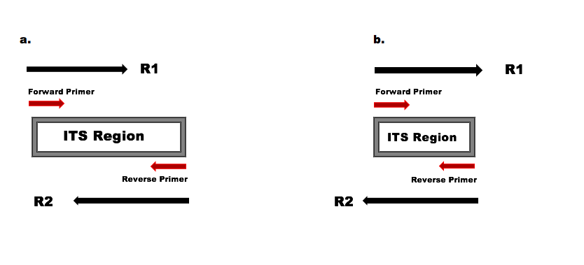
a) The amplified ITS region is longer than the read lengths, the forward and reverse reads overlap to capture the full amplified ITS region, but do not read into the opposite primer. b) The amplified ITS region is shorter than the read lengths, and the forward and reverse reads extend into the opposite primers which will appear in their reverse complement form towards the ends of those reads.
Because both scenarios pictured above typically occur within the same ITS dataset, a critical addition to ITS worfklows is the removal of primers on the forward and reverse reads, in a way that accounts for the possibility of read-through into the opposite primer. This is true even if the amplicon sequencing strategy doesn’t include the primers, as read-through into the opposite primer can still occur.
In the standard 16S workflow, it is generally possible to remove
primers (when included on the reads) via the trimLeft
parameter
(filterAndTrim(..., trimLeft=(FWD_PRIMER_LEN, REV_PRIMER_LEN)))
as they only appear at the start of the reads and have a fixed length.
However, the more complex read-through scenarios that are encountered
when sequencing the highly-length-variable ITS region require the use of
external tools. Here we present the cutadapt
tool for removal of primers from the ITS amplicon sequencing data.
Starting point
This workflow assumes that your sequencing data meets certain criteria:
- Samples have been demultiplexed, i.e., split into individual per-sample fastq files.
- If paired-end sequencing data, the forward and reverse fastq files contain reads in matched order.
You can also refer to the FAQ for recommendations for some common issues.
Getting ready
Along with the dada2 library, we also load the
ShortRead and the Biostrings package (R
Bioconductor packages; can be installed from the following locations, dada2,
ShortRead
and Biostrings)
which will help in identification and count of the primers present on
the raw FASTQ sequence files.
library(dada2)
packageVersion("dada2")
library(ShortRead)
packageVersion("ShortRead")
library(Biostrings)
packageVersion("Biostrings")
[1] '1.27.1'
[1] '1.56.1'
[1] '2.66.0'The dataset used here is the Amplicon sequencing library #1, an ITS Mock community constructed by selecting 19 known fungal cultures from the microbial culture collection at the USDA Agricultural Research Service (CFMR) culture collection and sequenced on an Illumina MiSeq using a version 3 (600 cycle) reagent kit.
To follow along, download the forward and reverse fastq files from the 31 samples listed in the ENA Project. Define the following path variable so that it points to the directory containing those files on your machine:
path <- "~/test/ITS_tutorial"  ## CHANGE ME to the directory containing the fastq files.
list.files(path)
[1] "cutadapt" "filtN" "SRR5314314_1.fastq.gz"
[4] "SRR5314314_2.fastq.gz" "SRR5314315_1.fastq.gz" "SRR5314315_2.fastq.gz"
[7] "SRR5314316_1.fastq.gz" "SRR5314316_2.fastq.gz" "SRR5314317_1.fastq.gz"
[10] "SRR5314317_2.fastq.gz" "SRR5314331_1.fastq.gz" "SRR5314331_2.fastq.gz"
[13] "SRR5314332_1.fastq.gz" "SRR5314332_2.fastq.gz" "SRR5314333_1.fastq.gz"
[16] "SRR5314333_2.fastq.gz" "SRR5314334_1.fastq.gz" "SRR5314334_2.fastq.gz"
[19] "SRR5314335_1.fastq.gz" "SRR5314335_2.fastq.gz" "SRR5314336_1.fastq.gz"
[22] "SRR5314336_2.fastq.gz" "SRR5314337_1.fastq.gz" "SRR5314337_2.fastq.gz"
[25] "SRR5314338_1.fastq.gz" "SRR5314338_2.fastq.gz" "SRR5314339_1.fastq.gz"
[28] "SRR5314339_2.fastq.gz" "SRR5314343_1.fastq.gz" "SRR5314343_2.fastq.gz"
[31] "SRR5314344_1.fastq.gz" "SRR5314344_2.fastq.gz" "SRR5314345_1.fastq.gz"
[34] "SRR5314345_2.fastq.gz" "SRR5314346_1.fastq.gz" "SRR5314346_2.fastq.gz"
[37] "SRR5314347_1.fastq.gz" "SRR5314347_2.fastq.gz" "SRR5314348_1.fastq.gz"
[40] "SRR5314348_2.fastq.gz" "SRR5314349_1.fastq.gz" "SRR5314349_2.fastq.gz"
[43] "SRR5314350_1.fastq.gz" "SRR5314350_2.fastq.gz" "SRR5314351_1.fastq.gz"
[46] "SRR5314351_2.fastq.gz" "SRR5314355_1.fastq.gz" "SRR5314355_2.fastq.gz"
[49] "SRR5314356_1.fastq.gz" "SRR5314356_2.fastq.gz" "SRR5314357_1.fastq.gz"
[52] "SRR5314357_2.fastq.gz" "SRR5314358_1.fastq.gz" "SRR5314358_2.fastq.gz"
[55] "SRR5314359_1.fastq.gz" "SRR5314359_2.fastq.gz" "SRR5314360_1.fastq.gz"
[58] "SRR5314360_2.fastq.gz" "SRR5314361_1.fastq.gz" "SRR5314361_2.fastq.gz"
[61] "SRR5314362_1.fastq.gz" "SRR5314362_2.fastq.gz" "SRR5314363_1.fastq.gz"
[64] "SRR5314363_2.fastq.gz"If the packages loaded successfully and your listed files match those here, your are ready to follow along with the ITS workflow.
Before proceeding, we will now do a bit of housekeeping, and generate
matched lists of the forward and reverse read files, as well as parsing
out the sample name. Here we assume forward and reverse read files are
in the format SAMPLENAME_1.fastq.gz and
SAMPLENAME_2.fastq.gz, respectively, so string parsing may
have to be altered in your own data if your filenamess have a different
format.
fnFs <- sort(list.files(path, pattern = "_1.fastq.gz", full.names = TRUE))
fnRs <- sort(list.files(path, pattern = "_2.fastq.gz", full.names = TRUE))
Identify primers
The BITS3 (forward) and B58S3 (reverse) primers were used to amplify this dataset. We record the DNA sequences, including ambiguous nucleotides, for those primers.
FWD <- "ACCTGCGGARGGATCA"  ## CHANGE ME to your forward primer sequence
REV <- "GAGATCCRTTGYTRAAAGTT"  ## CHANGE ME...
In theory if you understand your amplicon sequencing setup, this is sufficient to continue. However, to ensure we have the right primers, and the correct orientation of the primers on the reads, we will verify the presence and orientation of these primers in the data.
allOrients <- function(primer) {
    # Create all orientations of the input sequence
    require(Biostrings)
    dna <- DNAString(primer)  # The Biostrings works w/ DNAString objects rather than character vectors
    orients <- c(Forward = dna, Complement = Biostrings::complement(dna), Reverse = Biostrings::reverse(dna),
        RevComp = Biostrings::reverseComplement(dna))
    return(sapply(orients, toString))  # Convert back to character vector
}
FWD.orients <- allOrients(FWD)
REV.orients <- allOrients(REV)
FWD.orients
## Forward Complement Reverse RevComp
## "ACCTGCGGARGGATCA" "TGGACGCCTYCCTAGT" "ACTAGGRAGGCGTCCA" "TGATCCYTCCGCAGGT"The presence of ambiguous bases (Ns) in the sequencing reads makes accurate mapping of short primer sequences difficult. Next we are going to “pre-filter” the sequences just to remove those with Ns, but perform no other filtering.
fnFs.filtN <- file.path(path, "filtN", basename(fnFs)) # Put N-filtered files in filtN/ subdirectory
fnRs.filtN <- file.path(path, "filtN", basename(fnRs))
filterAndTrim(fnFs, fnFs.filtN, fnRs, fnRs.filtN, maxN = 0, multithread = TRUE)
We are now ready to count the number of times the primers appear in the forward and reverse read, while considering all possible primer orientations. Identifying and counting the primers on one set of paired end FASTQ files is sufficient, assuming all the files were created using the same library preparation, so we’ll just process the first sample.
primerHits <- function(primer, fn) {
    # Counts number of reads in which the primer is found
    nhits <- vcountPattern(primer, sread(readFastq(fn)), fixed = FALSE)
    return(sum(nhits > 0))
}
rbind(FWD.ForwardReads = sapply(FWD.orients, primerHits, fn = fnFs.filtN[[1]]), FWD.ReverseReads = sapply(FWD.orients,
    primerHits, fn = fnRs.filtN[[1]]), REV.ForwardReads = sapply(REV.orients, primerHits,
    fn = fnFs.filtN[[1]]), REV.ReverseReads = sapply(REV.orients, primerHits, fn = fnRs.filtN[[1]]))
Forward Complement Reverse RevComp
FWD.ForwardReads 4214 0 0 0
FWD.ReverseReads 0 0 0 3743
REV.ForwardReads 0 0 0 3590
REV.ReverseReads 4200 0 0 0As expected, the FWD primer is found in the forward reads in its forward orientation, and in some of the reverse reads in its reverse-complement orientation (due to read-through when the ITS region is short). Similarly the REV primer is found with its expected orientations.
Note: Orientation mixups are a common trip-up. If,
for example, the REV primer is matching the Reverse reads in its RevComp
orientation, then replace REV with its reverse-complement orientation
(REV <- REV.orient[["RevComp"]]) before proceeding.
Remove Primers
These primers can be now removed using a specialized primer/adapter removal tool. Here, we use cutadapt for this purpose. Download, installation and usage instructions are available online: http://cutadapt.readthedocs.io/en/stable/index.html
Install cutadapat if you don’t have it already. After installing cutadapt, we need to tell R the path to the cutadapt command.
cutadapt <- "/usr/local/bin/cutadapt" # CHANGE ME to the cutadapt path on your machine
system2(cutadapt, args = "--version") # Run shell commands from R
If the above command succesfully executed, R has found cutadapt and you are ready to continue following along.
We now create output filenames for the cutadapt-ed files, and define the parameters we are going to give the cutadapt command. The critical parameters are the primers, and they need to be in the right orientation, i.e. the FWD primer should have been matching the forward-reads in its forward orientation, and the REV primer should have been matching the reverse-reads in its forward orientation. Warning: A lot of output will be written to the screen by cutadapt!
path.cut <- file.path(path, "cutadapt")
if(!dir.exists(path.cut)) dir.create(path.cut)
fnFs.cut <- file.path(path.cut, basename(fnFs))
fnRs.cut <- file.path(path.cut, basename(fnRs))

FWD.RC <- dada2:::rc(FWD)
REV.RC <- dada2:::rc(REV)
# Trim FWD and the reverse-complement of REV off of R1 (forward reads)
R1.flags <- paste("-g", FWD, "-a", REV.RC)
# Trim REV and the reverse-complement of FWD off of R2 (reverse reads)
R2.flags <- paste("-G", REV, "-A", FWD.RC)
# Run Cutadapt
for(i in seq_along(fnFs)) {
  system2(cutadapt, args = c(R1.flags, R2.flags, "-n", 2, # -n 2 required to remove FWD and REV from reads
                             "-o", fnFs.cut[i], "-p", fnRs.cut[i], # output files
                             fnFs.filtN[i], fnRs.filtN[i])) # input files
}
As a sanity check, we will count the presence of primers in the first cutadapt-ed sample:
rbind(FWD.ForwardReads = sapply(FWD.orients, primerHits, fn = fnFs.cut[[1]]), FWD.ReverseReads = sapply(FWD.orients,
    primerHits, fn = fnRs.cut[[1]]), REV.ForwardReads = sapply(REV.orients, primerHits,
    fn = fnFs.cut[[1]]), REV.ReverseReads = sapply(REV.orients, primerHits, fn = fnRs.cut[[1]]))
Forward Complement Reverse RevComp
FWD.ForwardReads 0 0 0 0
FWD.ReverseReads 0 0 0 0
REV.ForwardReads 0 0 0 0
REV.ReverseReads 0 0 0 0Success! Primers are no longer detected in the cutadapted reads.
The primer-free sequence files are now ready to be analyzed through the DADA2 pipeline. Similar to the earlier steps of reading in FASTQ files, we read in the names of the cutadapt-ed FASTQ files and applying some string manipulation to get the matched lists of forward and reverse fastq files.
# Forward and reverse fastq filenames have the format:
cutFs <- sort(list.files(path.cut, pattern = "_1.fastq.gz", full.names = TRUE))
cutRs <- sort(list.files(path.cut, pattern = "_2.fastq.gz", full.names = TRUE))

# Extract sample names, assuming filenames have format:
get.sample.name <- function(fname) strsplit(basename(fname), "_")[[1]][1]
sample.names <- unname(sapply(cutFs, get.sample.name))
head(sample.names)
[1] "SRR5314314" "SRR5314315" "SRR5314316" "SRR5314317" "SRR5314331"
[6] "SRR5314332"Inspect read quality profiles
We start by visualizing the quality profiles of the forward reads:
plotQualityProfile(cutFs[1:2])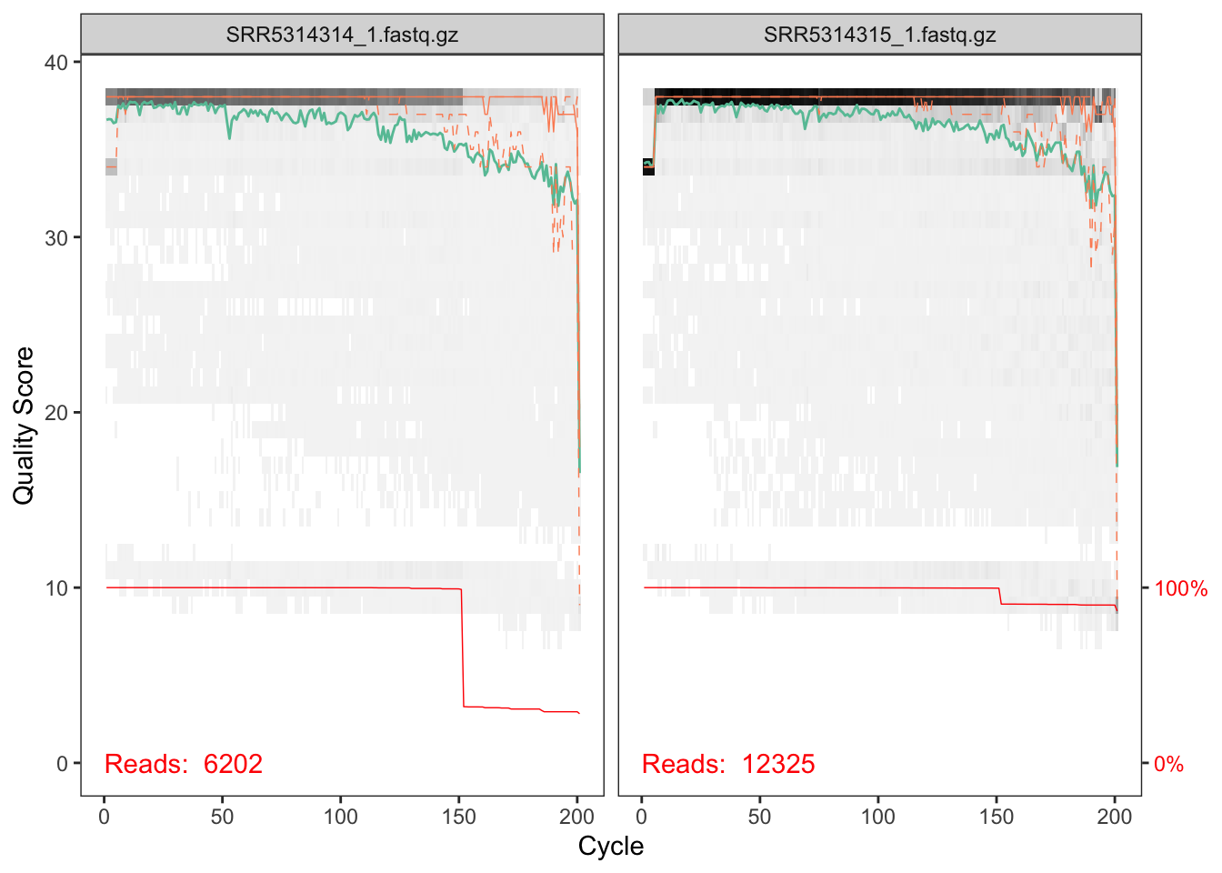
The quality profile plot is a gray-scale heatmap of the frequency of each quality score at each base position. The median quality score at each position is shown by the green line, and the quartiles of the quality score distribution by the orange lines. The red line shows the scaled proportion of reads that extend to at least that position.
The forward reads are of good quality. The red line shows that a significant chunk of reads were cutadapt-ed to about 150nts in length, likely reflecting the length of the amplified ITS region in one of the taxa present in these samples. Note that, unlike in the 16S Tutorial Workflow, we will not be truncating the reads to a fixed length, as the ITS region has significant biological length variation that is lost by such an appraoch.
Now we visualize the quality profile of the reverse reads:
plotQualityProfile(cutRs[1:2])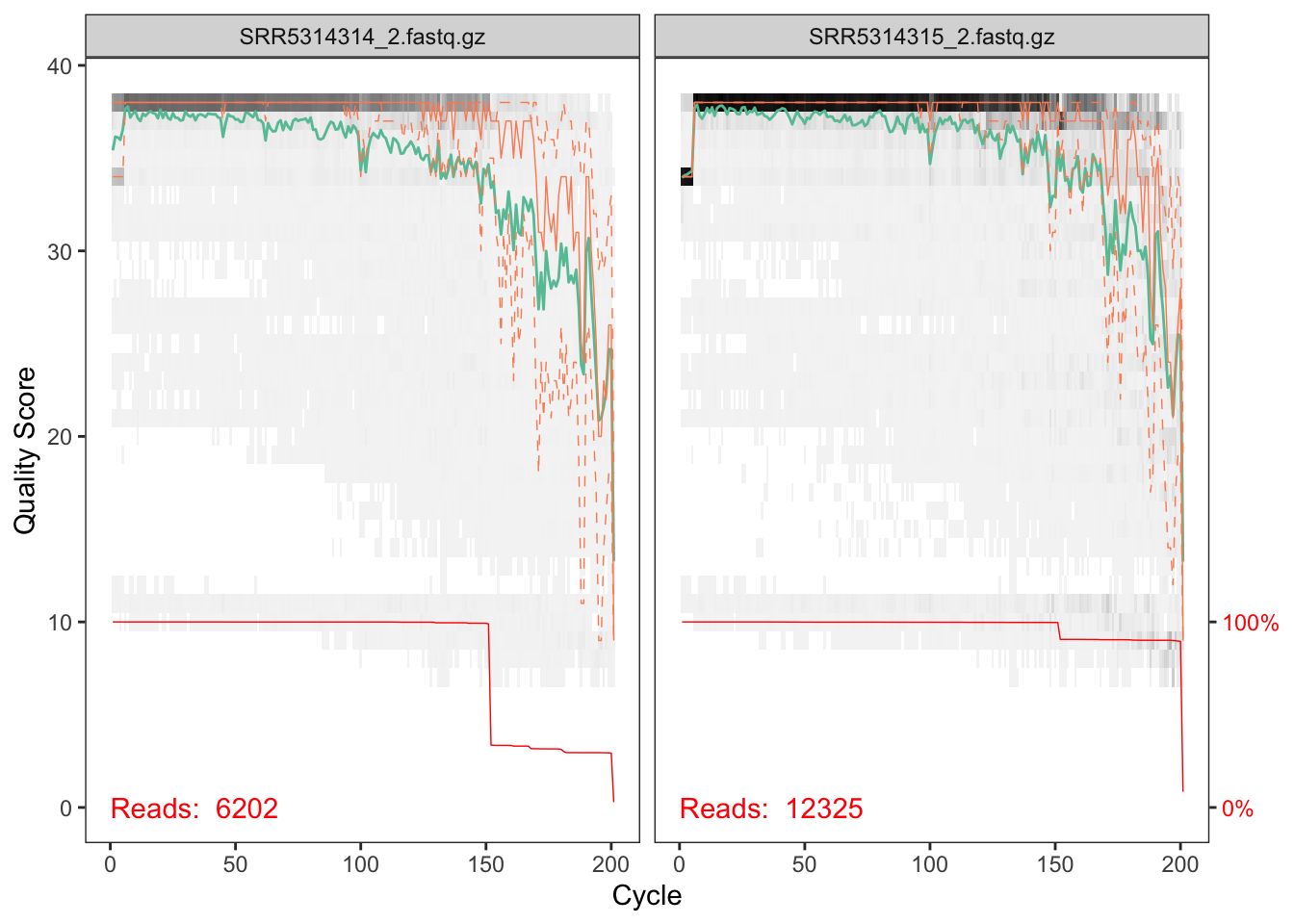
These reverse reads are of decent, but less good, quality. Note that we see the same length peak at around ~150nts, and in the same proportions, as we did in the forward reads. A good sign of consistency!
##Filter and trim
Assigning the filenames for the output of the filtered reads to be stored as fastq.gz files.
filtFs <- file.path(path.cut, "filtered", basename(cutFs))
filtRs <- file.path(path.cut, "filtered", basename(cutRs))
For this dataset, we will use standard filtering paraments:
maxN=0 (DADA2 requires sequences contain no Ns),
truncQ = 2, rm.phix = TRUE and
maxEE=2. The maxEE parameter sets the maximum
number of “expected errors” allowed in a read, which is a better
filter than simply averaging quality scores. Note:
We enforce a minLen here, to get rid of spurious very
low-length sequences. This was not needed in the 16S Tutorial Workflow
because truncLen already served that purpose.
out <- filterAndTrim(cutFs, filtFs, cutRs, filtRs, maxN = 0, maxEE = c(2, 2), truncQ = 2,
    minLen = 50, rm.phix = TRUE, compress = TRUE, multithread = TRUE)  # on windows, set multithread = FALSE
head(out)
reads.in reads.out
SRR5314314_1.fastq.gz 6202 5658
SRR5314315_1.fastq.gz 12325 10985
SRR5314316_1.fastq.gz 16006 14046
SRR5314317_1.fastq.gz 11801 10423
SRR5314331_1.fastq.gz 17399 15213
SRR5314332_1.fastq.gz 42604 36742
Learn the Error Rates
Please ignore all the “Not all sequences were the same length.” messages in the next couple sections. We know they aren’t, and it’s OK!
errF <- learnErrors(filtFs, multithread = TRUE)101352287 total bases in 624059 reads from 22 samples will be used for learning the error rates.errR <- learnErrors(filtRs, multithread = TRUE)100992324 total bases in 624059 reads from 22 samples will be used for learning the error rates.Visualize the estimated error rates as a sanity check.
plotErrors(errF, nominalQ = TRUE)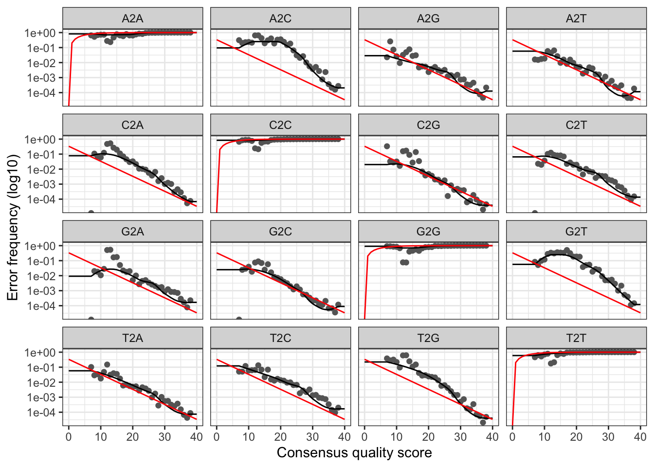
Everything looks reasonable and we proceed with confidence.
Sample Inference
At this step, the core sample inference algorithm is applied to the dereplicated data.
dadaFs <- dada(filtFs, err = errF, multithread = TRUE)
dadaRs <- dada(filtRs, err = errR, multithread = TRUE)
Merge paired reads
mergers <- mergePairs(dadaFs, filtFs, dadaRs, filtRs, verbose=TRUE)Construct Sequence Table
We can now construct an amplicon sequence variant table (ASV) table, a higher-resolution version of the OTU table produced by traditional methods.
seqtab <- makeSequenceTable(mergers)
dim(seqtab)
## [1] 31 549Remove chimeras
seqtab.nochim <- removeBimeraDenovo(seqtab, method="consensus", multithread=TRUE, verbose=TRUE)Inspect distribution of sequence lengths:
table(nchar(getSequences(seqtab.nochim)))
106 107 110 113 115 116 129 130 137 141 142 143 146 151 153 156 158 160 167 168
  1   1   1   3   1   1   1   1   1   1   1   1   1   3   1   1   2   1   1   2
174 178 181 185 188 195 197 199 207 212 224 230 248 262 289 290 291 292 293 294
  1   1   1   1   1   1   1   1   1   1   1   1   1   2   1   2   3 133   7   1
As expected, quite a bit of length variability in the the amplified ITS region.
Track reads through the pipeline
We now inspect the the number of reads that made it through each step in the pipeline to verify everything worked as expected.
getN <- function(x) sum(getUniques(x))
track <- cbind(out, sapply(dadaFs, getN), sapply(dadaRs, getN), sapply(mergers, getN),
    rowSums(seqtab.nochim))
# If processing a single sample, remove the sapply calls: e.g. replace
# sapply(dadaFs, getN) with getN(dadaFs)
colnames(track) <- c("input", "filtered", "denoisedF", "denoisedR", "merged", "nonchim")
rownames(track) <- sample.names
head(track)
input filtered denoisedF denoisedR merged nonchim
SRR5314314 6202 5658 5639 5594 5548 5016
SRR5314315 12325 10985 10890 10722 10462 6076
SRR5314316 16006 14046 14025 13901 13806 7264
SRR5314317 11801 10423 10389 10341 10217 5485
SRR5314331 17399 15213 15209 15209 15085 15085
SRR5314332 42604 36742 36722 36734 34972 34972Looks good! We kept the majority of our raw reads, and there is no over-large drop associated with any single step.
Assign taxonomy
DADA2 supports fungal taxonmic assignment using the UNITE database!
The DADA2 package provides a native implementation of the naive Bayesian
classifier method for taxonomic assignment. The
assignTaxonomy function takes as input a set of sequences
to ba classified, and a training set of reference sequences with known
taxonomy, and outputs taxonomic assignments with at least minBoot
bootstrap confidence. For fungal taxonomy, the General Fasta release
files from the UNITE ITS
database can be downloaded and used as the reference.
We also maintain formatted training fastas for the RDP training set, GreenGenes clustered at 97% identity, and the Silva reference database for 16S, and additional trainings fastas suitable for protists and certain specific environments have been contributed.
unite.ref <- "~/tax/sh_general_release_dynamic_s_all_29.11.2022.fasta"  # CHANGE ME to location on your machine
taxa <- assignTaxonomy(seqtab.nochim, unite.ref, multithread = TRUE, tryRC = TRUE)
UNITE fungal taxonomic reference detected.Inspecting the taxonomic assignments:
taxa.print <- taxa  # Removing sequence rownames for display only
rownames(taxa.print) <- NULL
head(taxa.print)
Kingdom Phylum Class
[1,] "k__Fungi" "p__Basidiomycota" "c__Tremellomycetes"
[2,] "k__Fungi" "p__Ascomycota" "c__Taphrinomycetes"
[3,] "k__Fungi" "p__Ascomycota" "c__Sordariomycetes"
[4,] "k__Fungi" "p__Ascomycota" "c__Dothideomycetes"
[5,] "k__Fungi" "p__Ascomycota" "c__Sordariomycetes"
[6,] "k__Fungi" "p__Mortierellomycota" "c__Mortierellomycetes"
Order Family Genus Species
[1,] "o__Filobasidiales" "f__Filobasidiaceae" "g__Naganishia" "s__albida"
[2,] "o__Taphrinales" "f__Protomycetaceae" "g__Saitoella" "s__complicata"
[3,] "o__Hypocreales" "f__Nectriaceae" "g__Fusarium" NA
[4,] "o__Pleosporales" "f__Pleosporaceae" "g__Alternaria" "s__tenuissima"
[5,] "o__Hypocreales" "f__Nectriaceae" "g__Fusarium" "s__graminearum"
[6,] "o__Mortierellales" "f__Mortierellaceae" "g__Podila" "s__humilis" Look like fungi!
Maintained by Benjamin Callahan (benjamin DOT j DOT callahan AT gmail DOT com)
Documentation License: CC-BY 4.0